For Clinical Labs
In today’s diagnostic landscape, laboratories must deliver fast, reliable, and cost-effective results despite staffing shortages, tighter regulations, and rising technical complexity.

When establishing the precision of a method, we are interested in the method’s ability to produce consistent results. Precision measures the closeness of agreement between measured values obtained by replicate measurements on the same or similar objects under specified conditions. How should we measure it?
There is practically always some variation in measured results compared with real values. It consists of systematic error (bias) and random error. Precision measures random error. In ANOVA protocol, it is divided into three components
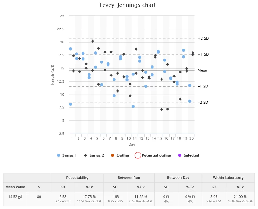
Image 1. Example data set with poor within-run precision.

Image 2. Example data set with poor between-run precision.
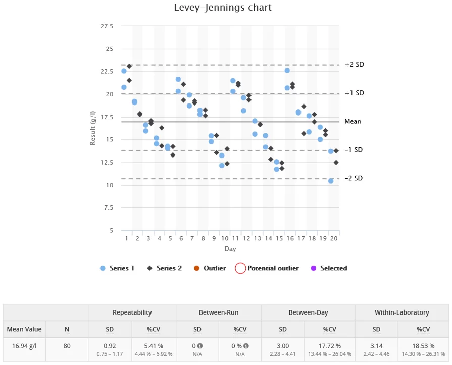
Image 3. Example data set with poor between-day precision
From these three components, you can obtain an estimate for within-laboratory precision that describes the measurement precision under usual operating conditions. The within-laboratory precision corresponds roughly to what can be estimated from a series of internal QC measurements.
If some of the above precision components dominate the results, you may be able to trace the reason behind this and sometimes even make it better, For this, the Levey-Jennings chart can be a valuable tool as it visualizes trends in the data set.
The example data sets in images 1, 2 and 3 show three fictional ANOVA protocols lasting for four weeks. Image 1 shows poor within-run precision, data shown in Image 2 has differences between morning and afternoon series (poor between-run precision), and Image 3 shows results falling from day to day during the work-week and increasing again after a weekend (poor between-day precision).
These are sort of extreme cases to show you what the graph can tell you. In real life, the effects are less evident, but if you know the instruments working cycles and what kind of samples are run on which days and who are performing which runs, etc., you can review the graphs to find out whether these things have a visible effect or not.
For validation purposes, we recommend following CLSI EP05-A3. For verification, a lighter procedure is enough, and EP15-A3 gives you guidance on that. You don’t need many samples, but you need to measure them many times.
It may feel surprising that you can get good results of within-run precision with only a couple of samples and daily replicates. The key is that you should use samples with relevant analyte concentrations. When establishing or verifying precision of a qualitative method, the sample should be near the limit of detection (LoD). For quantitative methods, you should design levels so that you can evaluate precision on high and low concentrations and near the medical decision point, which means that three samples are often enough.
If you conduct a 20-day ANOVA validation study with two daily series and two replicates, you get 40 replicate pairs of each sample that can be used for calculating within-run precision. Splitting measurements to many days and runs reflects usual operating parameters better, giving more credibility for the value obtained as within-run precision compared e.g., to a measurement setup with a couple of replicates of multiple samples all run at the same time. In addition, you have 40 runs to be used in evaluating between-run precision and results from 20 days to be used in evaluating between-day precision.
We know that some laboratories try to measure within-run precision and between-day precision separately (often called intra-assay and inter-assay precision), because it’s easier to collect daily control data to represent daily variance, and in addition gather one set of replicated patient samples to run together to measure within-run precision. As we have already mentioned, this procedure does not reflect normal operating parameters in an optimal way, and that’s why some relevant sources of error may go unnoticed.
But there’s also another reason for measuring all the precision components within one study. It’s the fact that you cannot remove the effect of within-run precision from a measurement setup, and therefore both the intra-assay and inter-assay measurements contain this error.
When you use the same measurement results for obtaining values for each component of precision, all these results are affected by same randomness. This makes these components statistically independent of each other. This means that you can compare them, and it is also possible to calculate the within-laboratory precision from them as the sum of squares.
It’s kind of like playing darts and trying to find out how well you are doing. Determining different precision components on different measurement setups would be a little bit like having a dartboard with straight stripes so that you would determine the position of a dart only in one dimension. If you turned the dartboard between game rounds, you would get information about both x and y values of the coordinates, but there would be no meaningful way to combine this information.
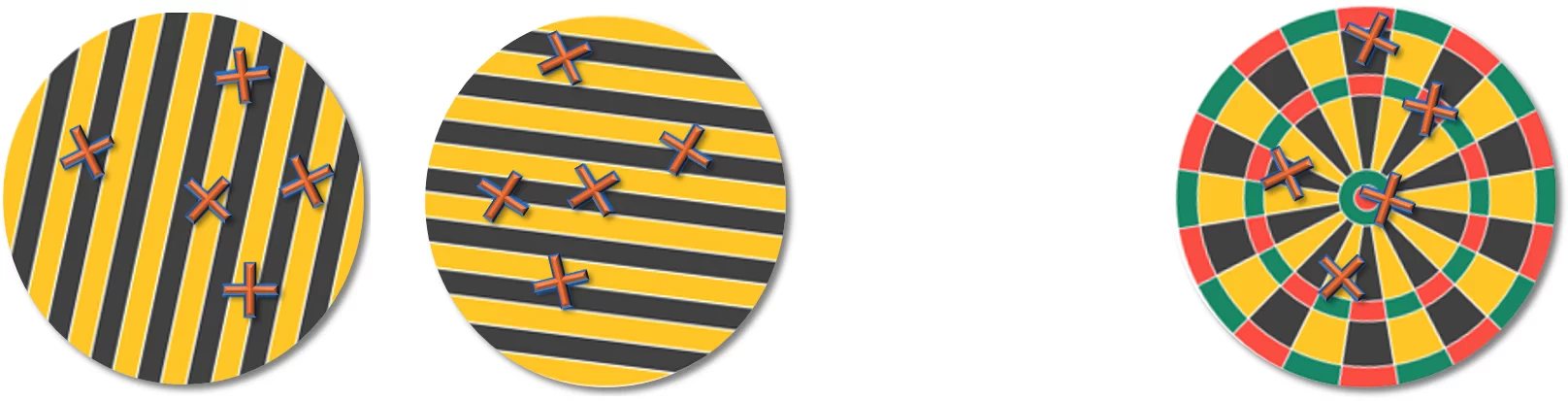
Image 4. On the left: measuring dart position in one dimension only on each play round. On the right: using a proper dartboard.
So similarly as you rather play darts using a proper dartboard, please establish your precision with a proper ANOVA protocol.
References